Linear Least Square and Ridge Regression
The package provides functions to perform Linear Least Square and Ridge Regression.
Linear Least Square
Linear Least Square is to find linear combination(s) of given variables to fit the responses by minimizing the squared error between them. This can be formulated as an optimization as follows:
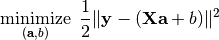
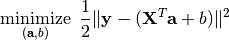
Sometimes, the coefficient matrix is given in a transposed form, in which case, the optimization is modified as:
The package provides llsq to solve these problems:
-
llsq(X, y; ...)¶ Solve the linear least square problem formulated above.
Here,
ycan be either a vector, or a matrix where each column is a response vector.This function accepts two keyword arguments:
trans: whether to use the transposed form. (default isfalse)bias: whether to include the bias termb. (default istrue)
The function results the solution
a. In particular, whenyis a vector (matrix),ais also a vector (matrix). Ifbiasis true, then the returned array is augmented as[a; b].
Examples
For a single response vector y (without using bias):
using MultivariateStats

# prepare data
X = rand(1000, 3)               # feature matrix
a0 = rand(3)                    # ground truths
y = X * a0 + 0.1 * randn(1000)  # generate response

# solve using llsq
a = llsq(X, y; bias=false)

# do prediction
yp = X * a

# measure the error
rmse = sqrt(mean(abs2(y - yp)))
print("rmse = $rmse")
For a single response vector y (using bias):
# prepare data
X = rand(1000, 3)
a0, b0 = rand(3), rand()
y = X * a0 + b0 + 0.1 * randn(1000)

# solve using llsq
sol = llsq(X, y)

# extract results
a, b = sol[1:end-1], sol[end]

# do prediction
yp = X * a + b'
For a matrix Y comprised of multiple columns:
# prepare data
X = rand(1000, 3)
A0, b0 = rand(3, 5), rand(1, 5)
Y = (X * A0 .+ b0) + 0.1 * randn(1000, 5)

# solve using llsq
sol = llsq(X, Y)

# extract results
A, b = sol[1:end-1,:], sol[end,:]

# do prediction
Yp = X * A .+ b'
Ridge Regression
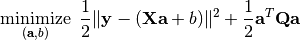
Compared to linear least square, Ridge Regression uses an additional quadratic term to regularize the problem:
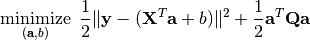
The transposed form:
The package provides ridge to solve these problems:
-
ridge(X, y, r; ...)¶ Solve the ridge regression problem formulated above.
Here,
ycan be either a vector, or a matrix where each column is a response vector.The argument
rgives the quadratic regularization matrixQ, which can be in either of the following forms:ris a real scalar, thenQis considered to ber * eye(n), wherenis the dimension ofa.ris a real vector, thenQis considered to bediagm(r).ris a real symmetric matrix, thenQis simply considered to ber.
This function accepts two keyword arguments:
trans: whether to use the transposed form. (default isfalse)bias: whether to include the bias termb. (default istrue)
The function results the solution
a. In particular, whenyis a vector (matrix),ais also a vector (matrix). Ifbiasis true, then the returned array is augmented as[a; b].